import pandas as pd
import datetime as dt
import numpy as np
import matplotlib.pyplot as plt
import pandas_datareader as pdr
import yfinance as yf

pd.options.mode.chained_assignment = None  # default='warn'

plt.style.use("ggplot")

Most of Technical Indicators used in quantitative trading are useless, the indicators introduced here are purely demonstrative purpose, they are mostly useless in trading practice.

Moving Average

Simple Moving Average

Simple moving average takes the formula \[ \begin{aligned} S M A_k & =\frac{p_{n-k+1}+p_{n-k+2} \cdots+p_n}{k} \\ & =\frac{1}{k} \sum_{i=n-k+1}^n p_i \end{aligned} \] Basically it calculates mean with a rolling window.

start_date = "2010-1-1"
end_date = dt.datetime.today()
usdjpy = pdr.data.DataReader(
    name="DEXJPUS", data_source="fred", start=start_date, end=end_date
).dropna()
usdjpy.columns = ["USDJPY"]

def get_sma(data, periods):
    sma = data.rolling(int(periods)).mean()
    return sma

usdjpy_sma50 = get_sma(data=usdjpy, periods=50)
usdjpy_sma252 = get_sma(data=usdjpy, periods=252)

fig, ax = plt.subplots(figsize=(20, 7))
ax.plot(usdjpy, label="USDJPY_Close")
ax.plot(usdjpy_sma50, label="SMA50")
ax.plot(usdjpy_sma252, label="SMA252")
ax.legend()
plt.show()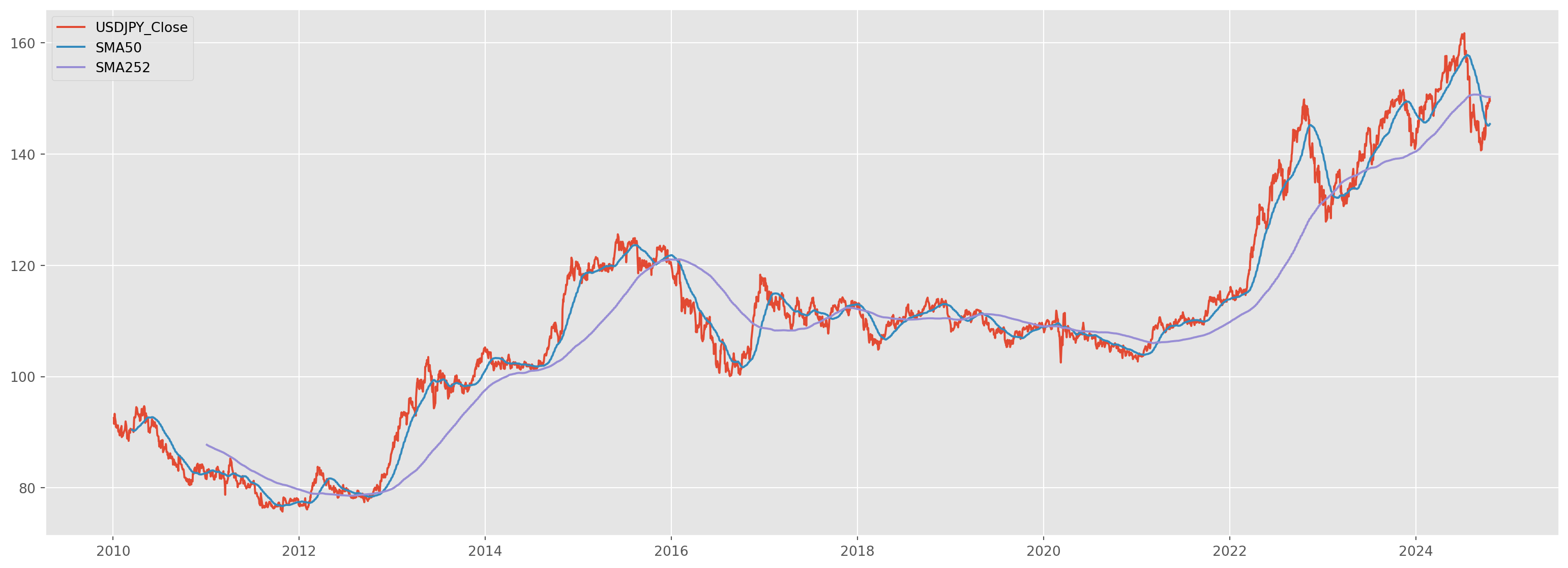

Exponential Moving Average

This is the formula of Exponential Moving Average

\[ \begin{gathered} K=\frac{2}{(n+1)} \\ E M A=K \cdot p+(1-K) \cdot E M A_{-1} \end{gathered} \]

The smoothing constant determines the weight to the most recent price, suppose your lag period is \(7\) \[ K= \frac{2}{7+1} \] \(K=.2\) means you give \(20\%\) weight to the most recent data.

n = np.arange(1, 101)
K = 2 / (n + 1)
fig, ax = plt.subplots(figsize=(12, 6))
ax.plot(n, K)
ax.set_ylabel("Lags")
ax.set_xlabel("Weight to Most Recent Data")
plt.show()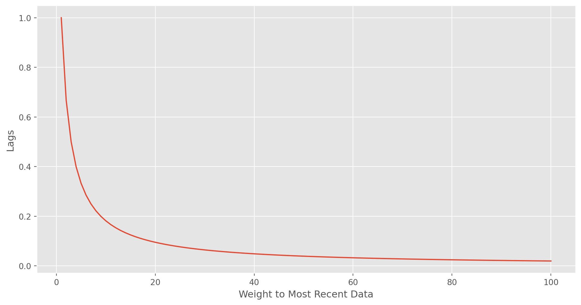

usdjpy_ema50 = usdjpy.ewm(span=50, min_periods=50).mean()

fig, ax = plt.subplots(figsize=(20, 7))
ax.plot(usdjpy[-600:], label="USDJPY_Close")
ax.plot(usdjpy_sma50[-600:], label="SMA50")
ax.plot(usdjpy_ema50[-600:], label="EMA50")
ax.legend()
plt.show()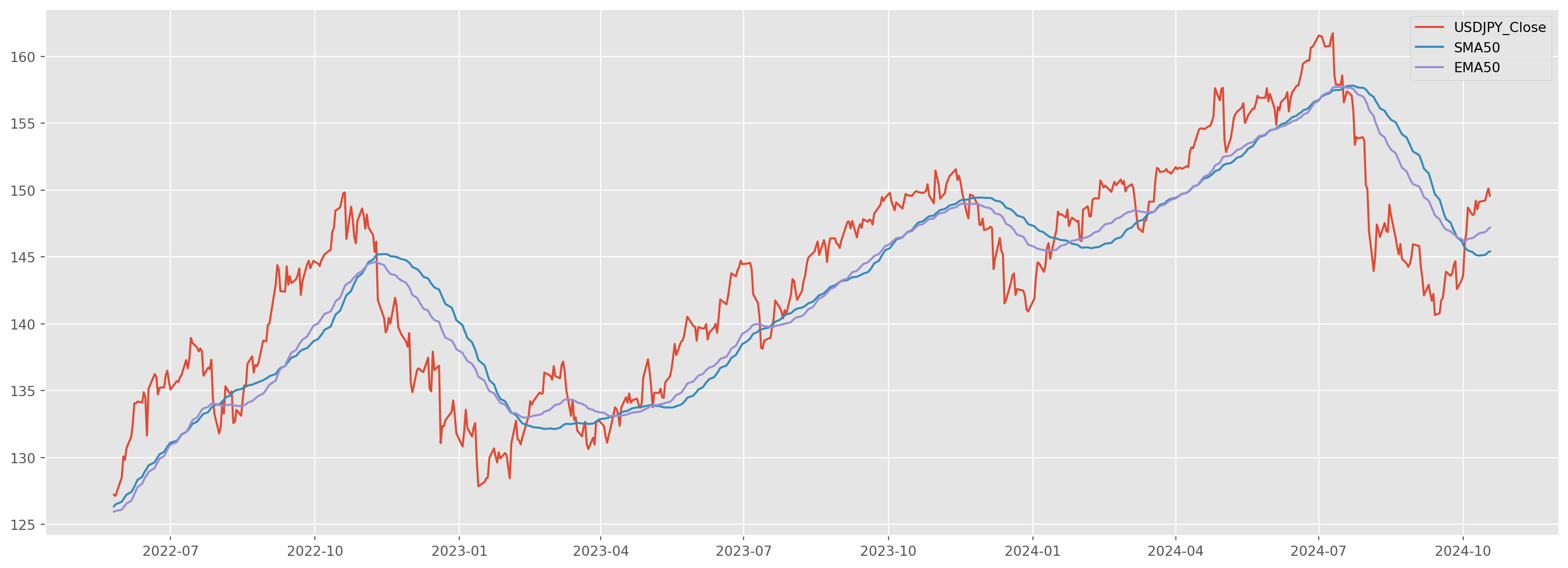

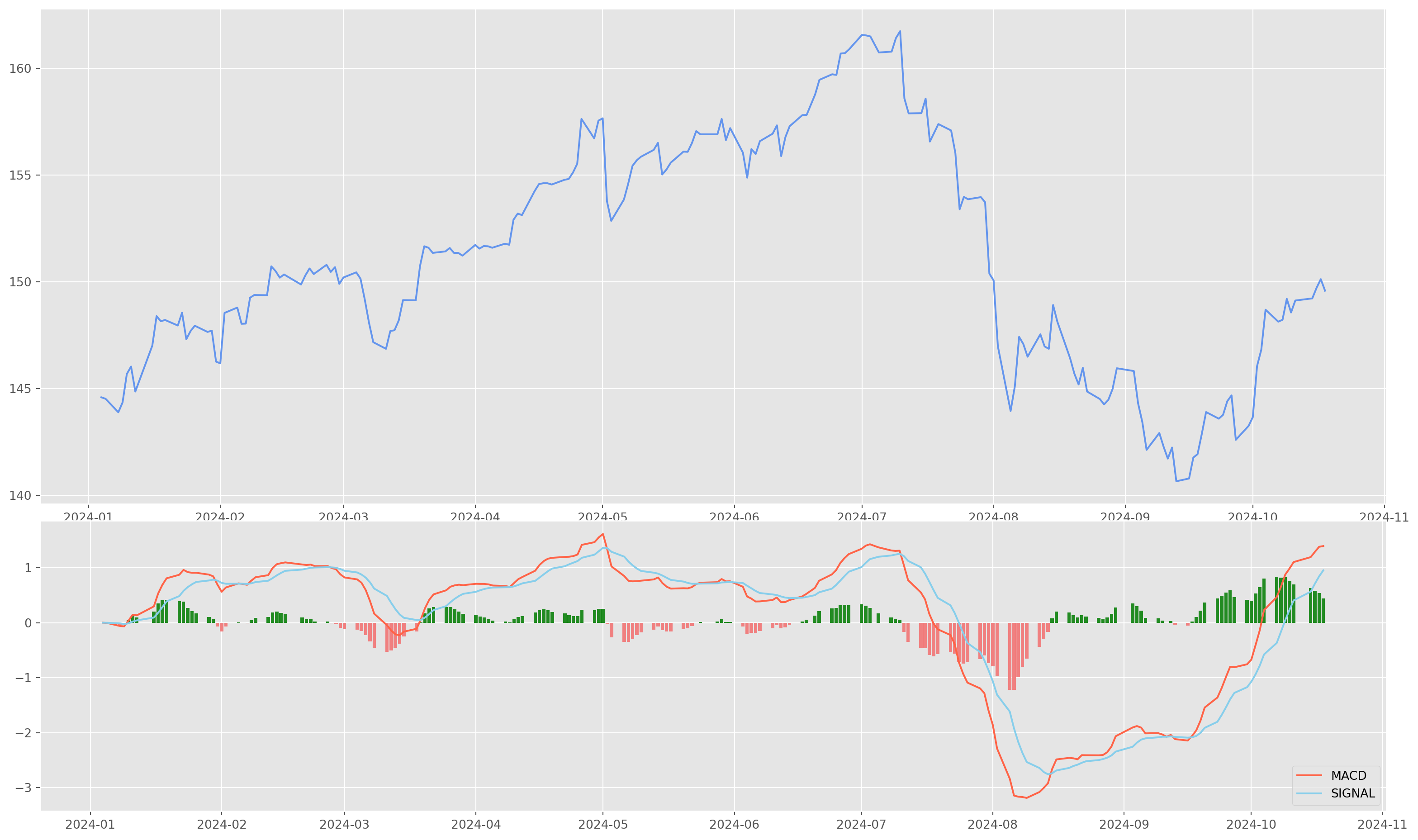
Moving Average Convergence/Divergence (MACD)

Formula of MACD is

\[ \begin{gathered} M A C D_p=E M A_{12}(p)-E M A_{26}(p) \\ S_{M A C D}=E M A_9(M A C D) \end{gathered} \]

def get_macd(price, slow, fast, smooth):
    fast = price.ewm(span=fast, adjust=False).mean()
    slow = price.ewm(span=slow, adjust=False).mean()
    macd = pd.DataFrame(fast - slow)
    signal = pd.DataFrame(macd.ewm(span=smooth, adjust=False).mean())
    hist = pd.DataFrame(macd - signal)
    frames = [macd, signal, hist]
    df = pd.concat(frames, join="inner", axis=1)
    df.columns = ["macd", "signal", "hist"]
    return df

def plot_macd(prices, macd, signal, hist):
    plt.figure(figsize=(20, 12))
    ax1 = plt.subplot2grid((8, 1), (0, 0), rowspan=5, colspan=1)
    ax2 = plt.subplot2grid((8, 1), (5, 0), rowspan=3, colspan=1)

    ax1.plot(prices, color="CornflowerBlue")
    ax2.plot(macd, color="tomato", linewidth=1.5, label="MACD")
    ax2.plot(signal, color="skyblue", linewidth=1.5, label="SIGNAL")

    # for i in range(len(prices)):
    #     if str(hist[i])[0] == '-':
    #         ax2.bar(prices.index[i], hist[i], color = 'LightCoral')
    #     else:
    #         ax2.bar(prices.index[i], hist[i], color = 'ForestGreen')

    for i in range(len(prices)):
        if hist[i] < 0:
            ax2.bar(prices.index[i], hist[i], color="LightCoral")
        else:
            ax2.bar(prices.index[i], hist[i], color="ForestGreen")

    plt.legend(loc="lower right")

jpy_set = usdjpy[-200:]
usdjpy_macd = get_macd(jpy_set, 26, 12, 9)
plot_macd(jpy_set, usdjpy_macd["macd"], usdjpy_macd["signal"], usdjpy_macd["hist"])

/tmp/ipykernel_4164/233838256.py:17: FutureWarning:

Series.__getitem__ treating keys as positions is deprecated. In a future version, integer keys will always be treated as labels (consistent with DataFrame behavior). To access a value by position, use `ser.iloc[pos]`

/tmp/ipykernel_4164/233838256.py:20: FutureWarning:

Series.__getitem__ treating keys as positions is deprecated. In a future version, integer keys will always be treated as labels (consistent with DataFrame behavior). To access a value by position, use `ser.iloc[pos]`

/tmp/ipykernel_4164/233838256.py:18: FutureWarning:

Series.__getitem__ treating keys as positions is deprecated. In a future version, integer keys will always be treated as labels (consistent with DataFrame behavior). To access a value by position, use `ser.iloc[pos]`

Bollinger Bands

The upper and lower Bollinger Bands are calculated by determining a simple moving average, and then adding/subtracting a specified number of standard deviations from the simple moving average to calculate the upper and lower bands.

\[ BB_{u} = SMA + d \sqrt{\frac{\sum_{i=1}^n(y_i-SMA)^2}{n}}\\ BB_{l} = SMA - d \sqrt{\frac{\sum_{i=1}^n(y_i-SMA)^2}{n}} \]

def get_bollinger_bands(prices, periods=20):
    sma = get_sma(prices, periods)
    std = prices.rolling(periods).std()
    bollinger_up = sma + std * 2
    bollinger_down = sma - std * 2
    return sma, bollinger_up, bollinger_down

periods = 20
jpy_sma, bollinger_up, bollinger_down = get_bollinger_bands(jpy_set, periods)

fig, ax = plt.subplots(figsize=(12, 6))
ax.plot(jpy_set, label="USDJPY")
ax.plot(bollinger_up)
ax.plot(bollinger_down)
ax.plot(jpy_sma, label="USDJPY_SMA_{}".format(periods))
ax.legend()
ax.set_title("Bollinger Bands")
plt.show()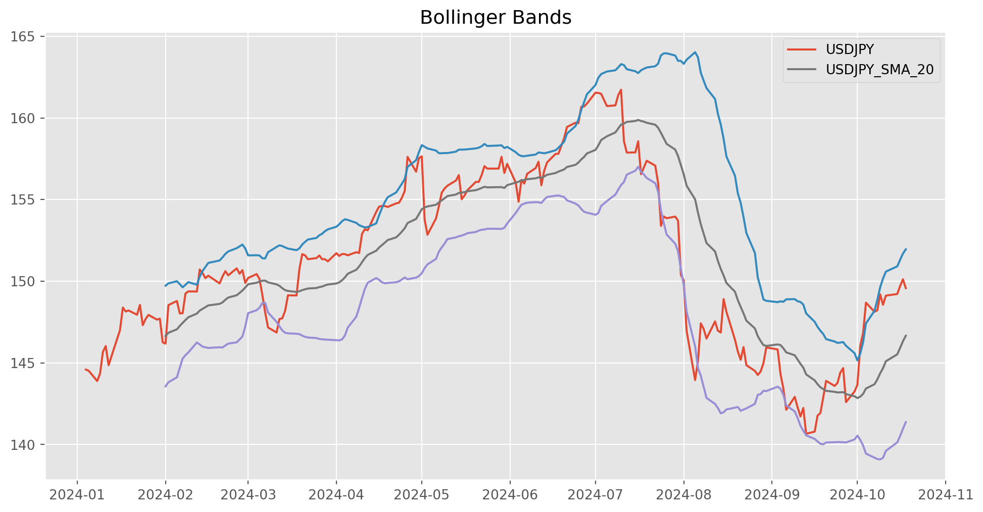

Average True Range

Average True Range (ATR) is the average of true ranges over the specified period. ATR measures volatility, taking into account any gaps in the price movement. Typically, the ATR calculation is based on 14 periods, which can be intraday, daily, weekly, or monthly.

Here’s the formula

\[ TR=\max{(H-L, |H-C_p|, |L-C_p|)}\\ ATR_t = \frac{ATR_{t-1}(n-1)+TR}{n} \]

To compute ATR, we need a full set an asset data with OLHC.

eurusd = yf.download(
    ["EURUSD=X"],
    start=dt.datetime.today() - dt.timedelta(days=1000),
    end=dt.datetime.today(),
    progress=True,
    actions="inline",
    interval="1d",
)
eurusd = eurusd.drop(["Adj Close", "Volume", "Dividends", "Stock Splits"], axis=1)

[*********************100%***********************]  1 of 1 completed

def get_atr(df, periods):
    df["H-L"] = df["High"] - df["Low"]
    df["H-Pc"] = abs(df["High"] - df["Close"].shift())
    df["L-Pc"] = abs(df["Low"] - df["Close"].shift())
    df["TR"] = df[["H-L", "H-Pc", "L-Pc"]].max(axis=1, skipna=False)
    # df['ATR'] = df['TR'].rolling(periods).mean()
    df["ATR"] = df["TR"].ewm(span=periods, adjust=False, min_periods=periods).mean()
    return df["ATR"]

atr_periods = 14
eurusd_atr = get_atr(eurusd, atr_periods)


def plot_atr(df):
    plt.figure(figsize=(20, 12))
    ax1 = plt.subplot2grid((8, 1), (0, 0), rowspan=5, colspan=1)
    ax2 = plt.subplot2grid((8, 1), (5, 0), rowspan=3, colspan=1)

    ax1.plot(df["Close"], color="CornflowerBlue", label="EURUSD")
    ax1.legend()
    ax2.plot(
        df["ATR"], color="tomato", linewidth=1.5, label="ATR {}".format(atr_periods)
    )
    ax2.legend()

plot_atr(eurusd)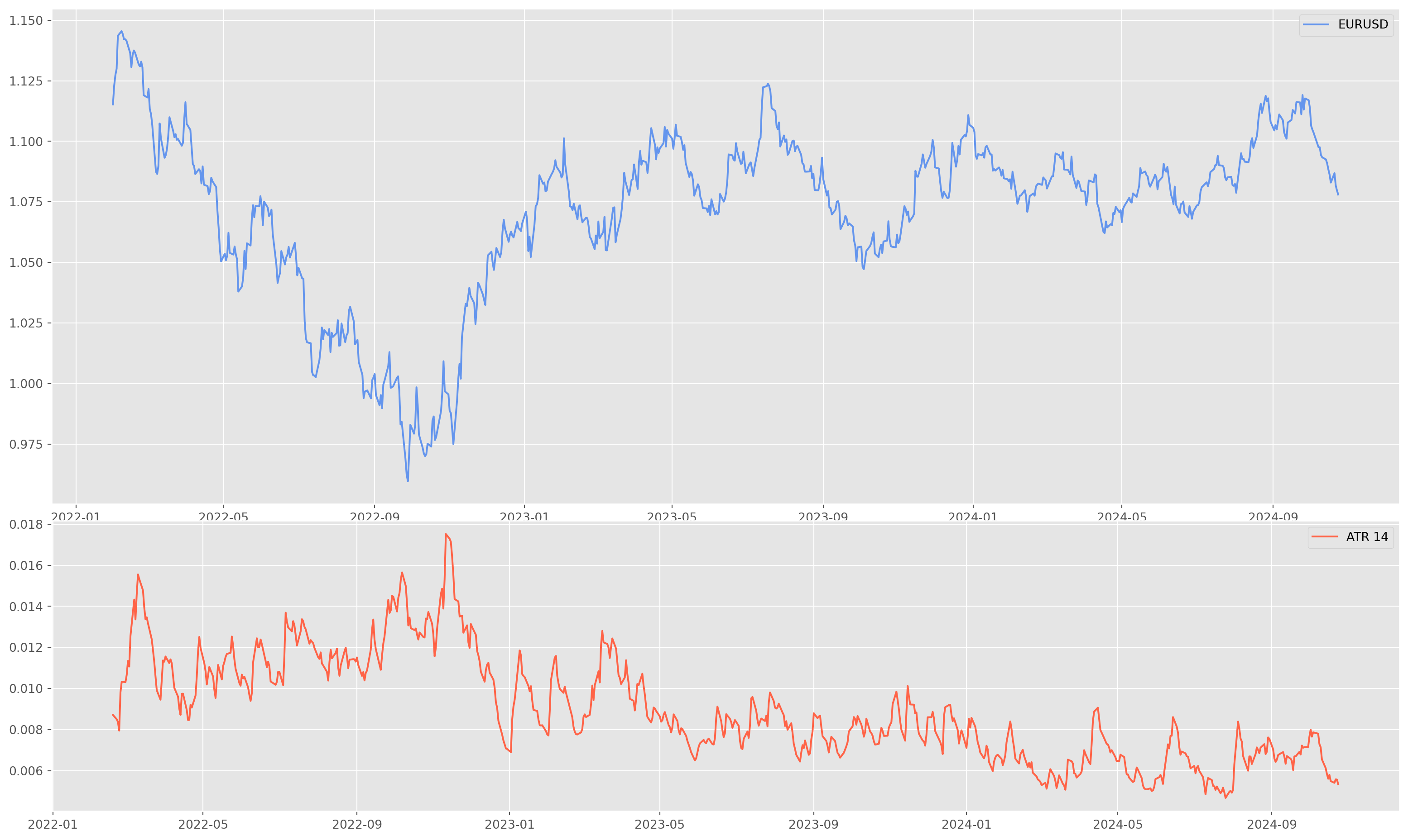

Relative Strength Index

The formula of RSI is

\[ RS = \frac{Avg. Gain}{Avg. Loss}\\ RSI = 100- \frac{100}{1+RS} \]

def get_rsi(df, periods=14, ema=True):
    """
    Returns a pd.Series with the relative strength index.
    """
    close_delta = df["Close"].diff()

    # Make two series: one for lower closes and one for higher closes
    up = close_delta.clip(
        lower=0
    )  # meaning that any value lower than 0, will be set to 0
    down = -1 * close_delta.clip(
        upper=0
    )  # meaning that any value more than 0, will be set to 0

    if ema == True:
        # Use exponential moving average
        avg_up = up.ewm(com=periods - 1, adjust=True, min_periods=periods).mean()
        avg_down = down.ewm(com=periods - 1, adjust=True, min_periods=periods).mean()
    else:
        # Use simple moving average
        avg_up = up.rolling(window=periods, adjust=False).mean()
        avg_down = down.rolling(window=periods, adjust=False).mean()

    rsi = avg_up / avg_down
    rsi = 100 - (100 / (1 + rsi))
    return rsi

rsi_periods = 14
eurusd_rsi = get_rsi(eurusd, periods=rsi_periods, ema=True)

def plot_rsi(df, rsi):
    plt.figure(figsize=(20, 12))
    ax1 = plt.subplot2grid((8, 1), (0, 0), rowspan=5, colspan=1)
    ax2 = plt.subplot2grid((8, 1), (5, 0), rowspan=3, colspan=1)

    ax1.plot(df["Close"], color="CornflowerBlue", label="EURUSD")
    ax1.legend()
    ax2.plot(rsi, color="tomato", linewidth=1.5, label="RSI {}".format(rsi_periods))
    ax2.axhline(70, ls="--", color="grey")
    ax2.axhline(30, ls="--", color="grey")
    ax2.fill_between(eurusd.index, 70, 30, color="DeepSkyBlue", alpha=0.1)
    ax2.legend()

plot_rsi(eurusd, eurusd_rsi)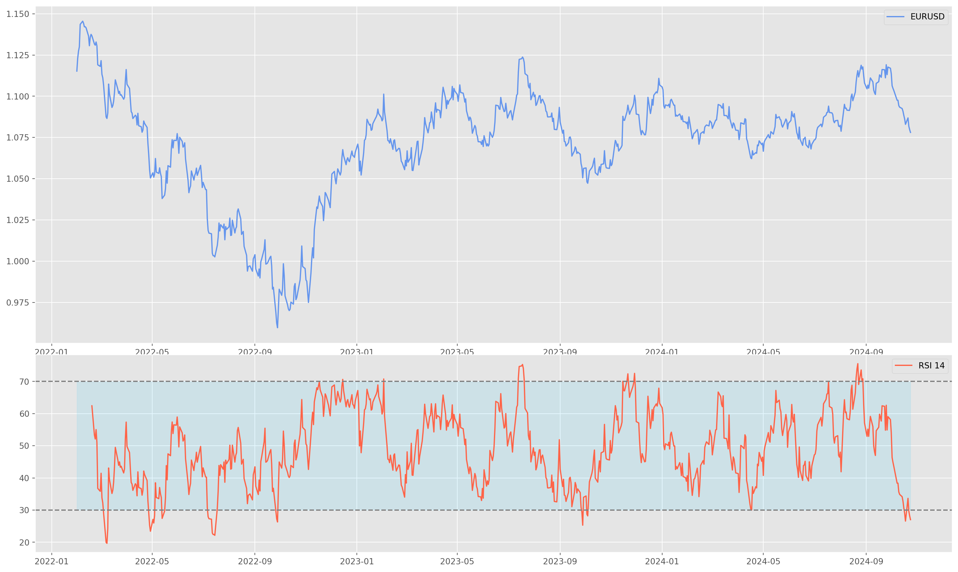

Average Directional Index

\[ \begin{aligned} +\mathrm{DI} & =\left(\frac{\text { Smoothed }+\mathrm{DM}}{\mathrm{ATR}}\right) \times 100 \\ -\mathrm{DI} & =\left(\frac{\text { Smoothed }-\mathrm{DM}}{\mathrm{ATR}}\right) \times 100 \\ \mathrm{DX} & =\left(\frac{|+\mathrm{DI}--\mathrm{DI}|}{|+\mathrm{DI}+-\mathrm{DI}|}\right) \times 100 \\ \mathrm{ADX} & =\frac{(\text { Prior ADX } \times 13)+\text { Current ADX }}{14} \end{aligned} \]

\(\text{DM}\) means directional movement, calculated by current high minus previous high, i.e. \(H_t - H_{t-1} = + \text{DM}\) or \(L_t - L_{t-1} = - \text{DM}\)

lulu = yf.download(
    ["LULU"],
    start=dt.datetime.today() - dt.timedelta(days=1000),
    end=dt.datetime.today(),
    progress=True,
    actions="inline",
    interval="1d",
)

[*********************100%***********************]  1 of 1 completed

def get_adx(df, periods):
    plus_dm = df["High"].diff()
    minus_dm = df["Low"].diff()
    plus_dm = plus_dm.clip(lower=0)
    minus_dm = minus_dm.clip(upper=0)
    df["H-L"] = df["High"] - df["Low"]
    df["H-Pc"] = abs(df["High"] - df["Close"].shift())
    df["L-Pc"] = abs(df["Low"] - df["Close"].shift())
    df["TR"] = df[["H-L", "H-Pc", "L-Pc"]].max(axis=1, skipna=False)
    df["ATR"] = df["TR"].ewm(span=periods, adjust=False, min_periods=periods).mean()

    plus_di = 100 * (plus_dm.ewm(alpha=1 / periods).mean() / df["ATR"])
    minus_di = abs(100 * (minus_dm.ewm(alpha=1 / periods).mean() / df["ATR"]))
    dx = (abs(plus_di - minus_di) / abs(plus_di + minus_di)) * 100
    adx = ((dx.shift(1) * (periods - 1)) + dx) / periods
    adx_smooth = adx.ewm(alpha=1 / periods).mean()
    return plus_di, minus_di, adx, adx_smooth

adx_periods = 14
plus_di, minus_di, adx, adx_smooth = get_adx(df=lulu, periods=adx_periods)

def plot_adx(df, adx, adx_smooth, adx_periods):
    plt.figure(figsize=(20, 12))
    ax1 = plt.subplot2grid((8, 1), (0, 0), rowspan=5, colspan=1)
    ax2 = plt.subplot2grid((8, 1), (5, 0), rowspan=3, colspan=1)

    ax1.plot(df["Close"], color="CornflowerBlue", label="LULU")
    ax1.legend()
    ax2.plot(
        adx,
        color="tomato",
        linewidth=1.5,
        label="ADX unsmoothed {}".format(adx_periods),
    )
    ax2.plot(
        adx_smooth,
        color="Brown",
        linewidth=1.5,
        label="ADX smoothed {}".format(adx_periods),
    )
    ax2.legend()
    plt.show()

plot_adx(lulu, adx, adx_smooth, adx_periods)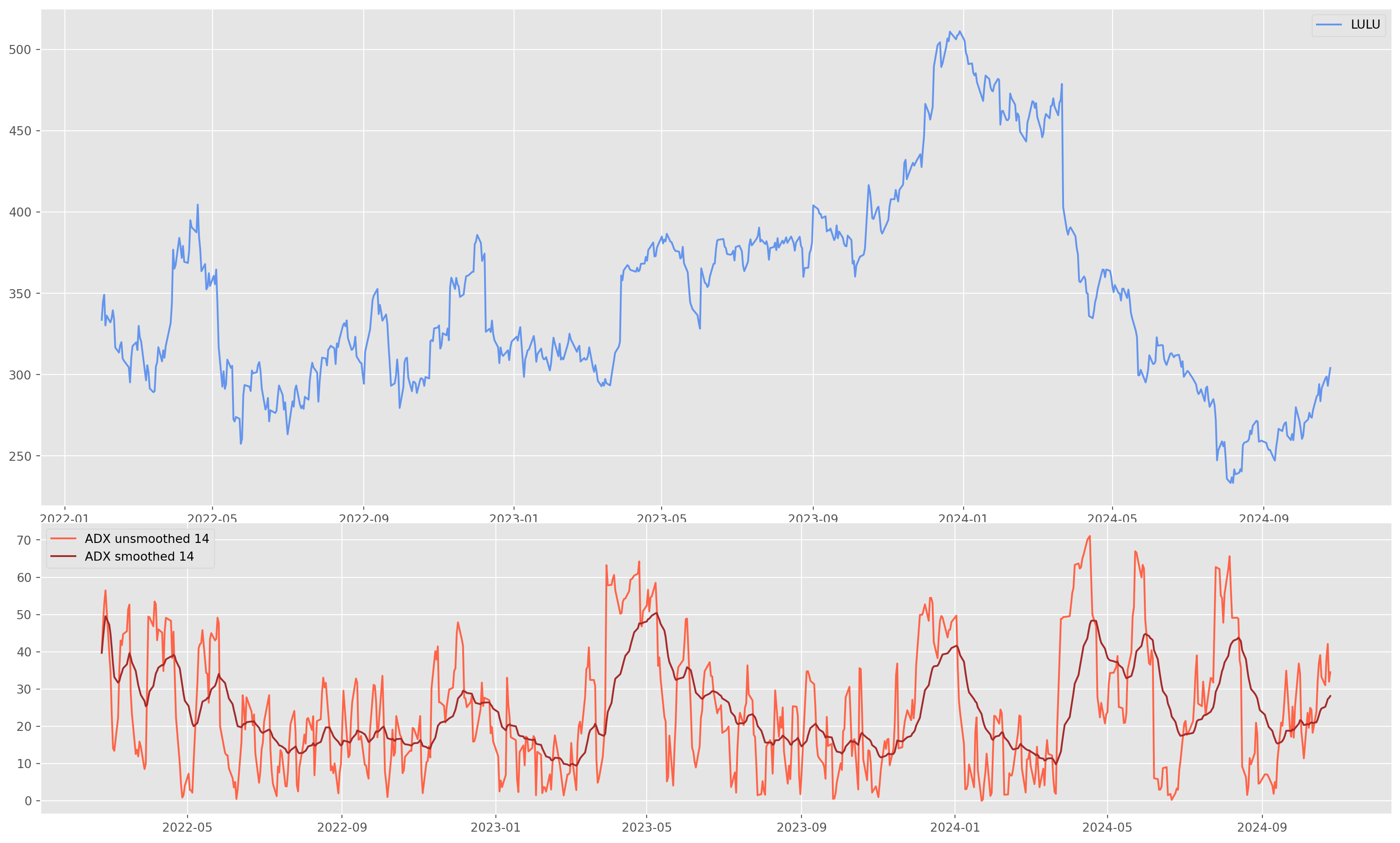

On-Balance Volume

As its name suggests, \(\text{OBV}\) is using trading volume to measure the money in-flow or out-flow into a certain asset.

\[ \mathrm{OBV}_t=\mathrm{OBV}_{t-1 }+ \begin{cases}\text { volume, } & \text { if }C_t>C_{t-1} \\ 0, & \text { if }C_t=C_{t-1} \\ -\text {volume, } & \text { if }C_t<C_{t-1}\end{cases} \] where: \[ C\text{ is close price}\\ \text{volume $=$ Latest trading volume amount} \]

As a reminder of np.where(condition, [x, y]), this says is that if condition holds True for some element in our array, the new array will choose elements from \(x\), otherwise \(y\), which is a convenient way to convert a data into dummy variables.

obv_periods = 21


def get_obv(df, periods):
    df_temp = (
        df.copy()
    )  # if you don't to change the original dataset after running the function, use a copy
    df_temp["Daily_ret"] = df_temp["Adj Close"].pct_change()
    df_temp["Direction"] = np.where(
        df_temp["Daily_ret"] >= 0, 1, -1
    )  # meaning that positive return indexed as 1, negative rturn indexed as 0
    df_temp["Direction"][0] = 0  # mannual assign the first value as 0
    df_temp["Volume_adj"] = df_temp["Volume"] * df_temp["Direction"]
    df_temp["OBV"] = df_temp["Volume_adj"].cumsum()
    return df_temp["OBV"]

obv = get_obv(lulu, obv_periods)

/tmp/ipykernel_4164/2972755750.py:12: FutureWarning:

ChainedAssignmentError: behaviour will change in pandas 3.0!
You are setting values through chained assignment. Currently this works in certain cases, but when using Copy-on-Write (which will become the default behaviour in pandas 3.0) this will never work to update the original DataFrame or Series, because the intermediate object on which we are setting values will behave as a copy.
A typical example is when you are setting values in a column of a DataFrame, like:

df["col"][row_indexer] = value

Use `df.loc[row_indexer, "col"] = values` instead, to perform the assignment in a single step and ensure this keeps updating the original `df`.

See the caveats in the documentation: https://pandas.pydata.org/pandas-docs/stable/user_guide/indexing.html#returning-a-view-versus-a-copy


/tmp/ipykernel_4164/2972755750.py:12: FutureWarning:

Series.__setitem__ treating keys as positions is deprecated. In a future version, integer keys will always be treated as labels (consistent with DataFrame behavior). To set a value by position, use `ser.iloc[pos] = value`

def plot_obv(df, obv):
    plt.figure(figsize=(20, 12))
    ax1 = plt.subplot2grid((8, 1), (0, 0), rowspan=5, colspan=1)
    ax2 = plt.subplot2grid((8, 1), (5, 0), rowspan=3, colspan=1)

    ax1.plot(df["Close"], color="CornflowerBlue", label="LULU")
    ax1.legend()
    ax2.plot(adx, color="tomato", linewidth=1.5, label="OBV {}".format(obv_periods))
    ax2.legend()
    plt.show()

plot_obv(lulu, 21)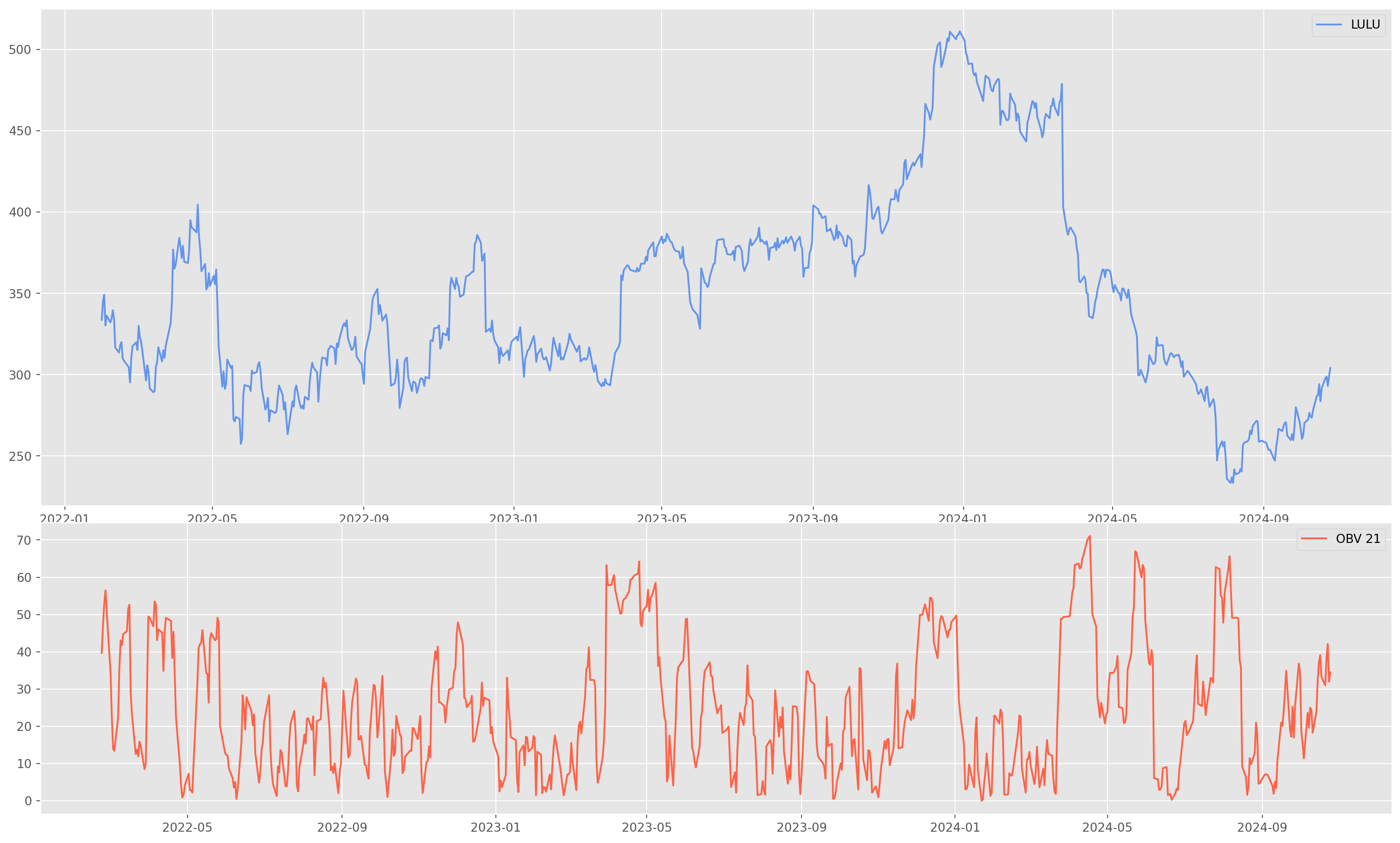

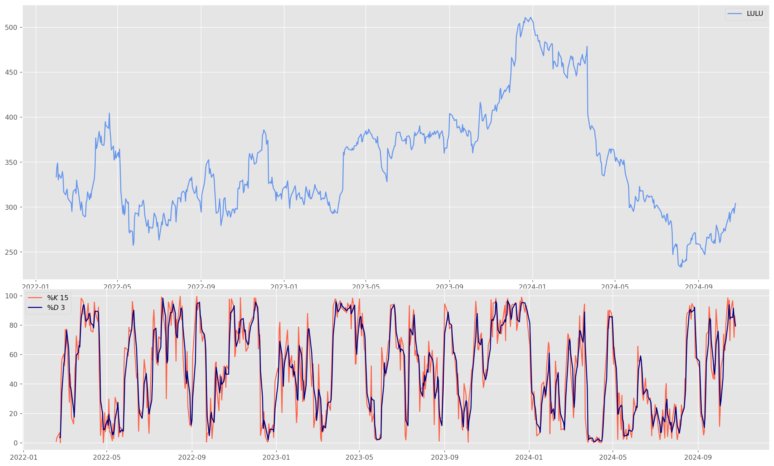
Stochastic Oscillators

Similar to RSI, SO also gives indication of overbought and oversold. Formula as below \[ \% K = \frac{C-L_n}{H_n - L_n}\times 100 \] where \(C\) is the current closing price, \(L_n\) is the lowest price in recent \(n\) period, the default setting \(n=15\). And \(\%D\) is just the mean value of \(\%K\). \[ \% D = \frac{1}{d}\sum_{i=i}^d \%K_i \] where by default \(d=3\).

Common ways of using Stochastic Oscillator: 1. Overbought/Oversold indicates potential reversal 2. Crossover of \(\%K\) and \(\%D\) 3. Divergence between price and oscillator indicates potential reversal

k_periods = 14
d_periods = 3


def get_stoc_oslr(df, k_periods, d_periods):
    df_temp = df.copy()
    df_temp["n-high"] = df_temp["High"].rolling(k_periods).max()
    df_temp["n-low"] = df_temp["Low"].rolling(k_periods).min()
    df_temp["%K"] = (
        (df_temp["Close"] - df_temp["n-low"])
        * 100
        / (df_temp["n-high"] - df_temp["n-low"])
    )
    df_temp["%D"] = df_temp["%K"].rolling(d_periods).mean()
    return df_temp["%K"], df_temp["%D"]

def plot_stoc_oslr(df, K_perc, D_perc, k_periods, d_periods):
    plt.figure(figsize=(20, 12))
    ax1 = plt.subplot2grid((8, 1), (0, 0), rowspan=5, colspan=1)
    ax2 = plt.subplot2grid((8, 1), (5, 0), rowspan=3, colspan=1)

    ax1.plot(df["Close"], color="CornflowerBlue", label="LULU")
    ax1.legend()
    ax2.plot(K_perc, color="tomato", linewidth=1.5, label=r"$\%K$ {}".format(k_periods))
    ax2.plot(D_perc, color="Navy", linewidth=1.5, label=r"$\%D$ {}".format(d_periods))
    ax2.legend()
    plt.show()

K_perc, D_perc = get_stoc_oslr(lulu, k_periods, d_periods)
plot_stoc_oslr(lulu, K_perc, D_perc, 15, 3)